Simulating Raman Fiber Amplifiers in Julia: From Theory to High-Performance Code

🚀 What You’ll Learn in This Post

A quick primer on Raman fiber amplifiers and their role in modern optical communication systems.
The physics and equations behind Raman gain and signal-pump interactions.
How to simulate Raman amplifiers using Julia programming language for high-performance computing.
Techniques to optimize Julia code using StaticArrays, in-place operations, and memory-efficient design.
Visual plot of power evolution along the fiber length.
Benchmarking results comparing Julia vs Python for scientific simulations.
Access to Julia code snippets, explanations, and performance tips for hands-on learning.

🤔 What is Raman fiber amplifier, and why simulate it?

A Raman fiber amplifier (RFA) uses the Raman scattering effect to amplify optical signals directly within the transmission fiber itself. Unlike traditional fiber amplifiers that require special dopants in optical fiber, Raman scattering can turn any ordinary optical fiber into an amplifier, making RFAs incredibly versatile for telecommunications systems.

Here are some of the points why RFAs are revolutionary:

Wavelength flexibility: Raman amplification can be done at any wavelength and in any conventional optical fiber.
Broad bandwidth: Leads to amplification of large range of wavelengths, essential for dense wavelength division multiplexing (WDM) systems
Distributed amplification: The entire fiber becomes the gain medium, providing amplification along the transmission path

RFAs are now commonly used in long-haul communication systems that are designed to operate over thousands of kilometers. Simulating these RFAs is crucial, as complex nonlinear interactions between pump and signal beams makes analytical solutions impossible for a practical situation. By modeling the coupled ordinary differential equations (ODE) that govern Raman amplification, we can optimize several aspects of the amplifier design such as pump parameters, fiber lengths, and design systems before performing an expensive experimental validation. Also simulation provides us a handy tool to understand the workings of a system by varying only the desired parameter, which is not possible in a practical system. Now let’s discuss why Julia programming language is a good choice to do the simulation.

🤷‍♂️ Why Julia?

Julia is uniquely positioned for scientific simulations like RFAs. Here are some of the reasons:

Performance: With Julia, one can achieve C-like speeds while having Python-like readability. For iterative ODE solving required in RFA simulations, this can lead to dramatically faster computation times—often 10-100x faster than Python
Simplicity: The syntax is intuitive for scientists and engineers. For example, one can write dPₚ = gR*Pₚ*Pₛ - αₛ*Pₛ and it looks exactly like the mathematical equation
Rich Ecosystem: DifferentialEquations.jl is, IMO, the most sophisticated ODE solver suite in any language, with over 200 methods for solving variety of differential equations, with a focus on speed and flexibility
Scientific Focus: Julia was designed from the ground up for numerical and scientific computing. It handles the “two-language problem” where one develop the prototype in a high-level language (eg: Python, MATLAB) but implement the main computation in a low-level language for performance (C, FORTRAN).

📘 Basic theory Refresher

Now before we dive deeper into writing the codes, lets discuss the theory a bit.

Brief overview of Raman amplification

When light interacts with molecular vibrations in glass, there can be transfer of energy between different wavelengths. This is known as Raman scattering. Imagine a high energy photon (pump) that collide with vibrating fiber molecules (phonons), giving up some of their energy becoming a lower energy photon (Stokes) at lower frequency or longer wavelength (The pump photons can also receive energy from phonons leading to higher frequency anti-Stokes photons, but this is usually a weak process at room temperatures). If a signal photon is already present at Stokes frequency, it can lead to stimulated Raman scattering leading to amplification of the signal wave at Stokes frequency (and thus Raman gain).

The power-balance equation

The heart of Raman amplifier simulation lies in two coupled ordinary differential equations (ODEs) that describe how pump and signal (Stokes) powers evolve along the fiber [1], [2] \[ \begin{align} \\ &\mathbf{Signal\ equation:} &\frac{dP_{s}}{dz}&= g_{R}P_{p}P_{s} - \alpha_{s}P_{s} \\ &\mathbf{Pump\ equation:} &\frac{dP_{p}}{dz}&= -\frac{\nu_{p}}{\nu_{s} }g_{R}P_{p}P_{s} - \alpha_{p}P_{p} \end{align} \tag{1}\] where:

\(P_{s}\) and \(P_{p}\) are signal and pump powers that are a function of position \(z\)
\(g_{R}\) is the Raman gain efficiency
\(\alpha_{s}\) and \(\alpha_{p}\) are signal and pump attenuation coefficients
\(\nu_{s}\) and \(\nu_{p}\) are signal and pump frequencies

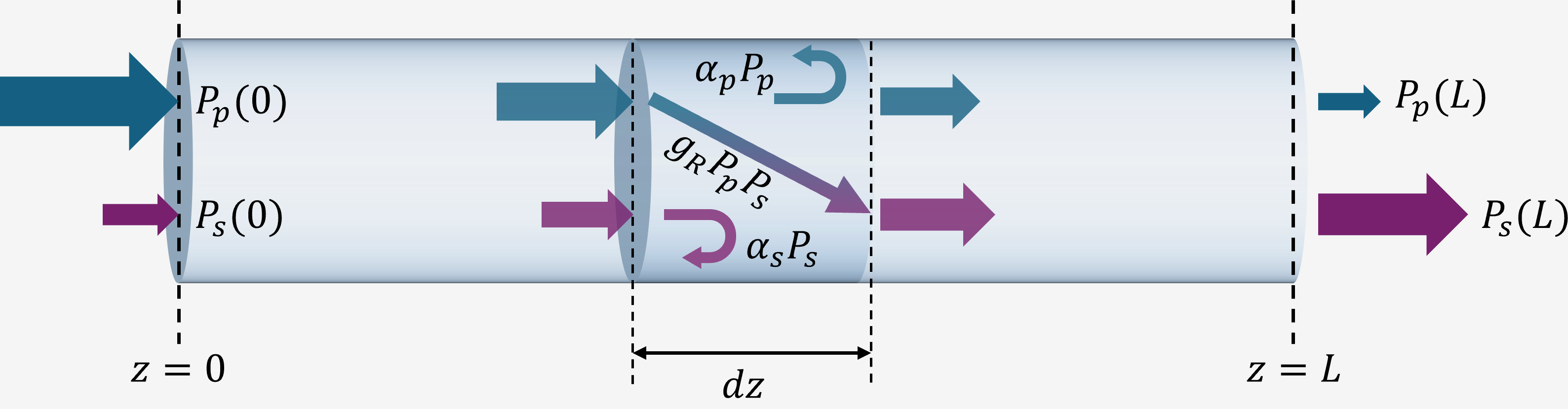
The \(g_{R}P_{p}P_{s}\) term is the power transfer from pump to signal due to stimulated Raman scattering and the term \(-\frac{\nu_{p}}{\nu_{s} }g_{R}P_{p}P_{s}\) represents the power loss in the pump as it is transferred to signal. The reason of the \(\nu_{p}/\nu_{s}\) term is due to photon number conservation (in absence of loss) [1].

The power-balance equations describes the initial pump and signal power \(P_{p}(0)\) and \(P_{s}(0)\) evolves along the fiber length \(L\).

Key assumptions

The above equations are derived with these assumptions

CW or quasi-CW regime: both pump and signal assumed to be close to continuous-wave(CW) and so no time dependence is considered, valid assumption in most telecommunications applications.
Single-mode fiber: both pump and signal waves are in the fundamental mode of fiber, appropriate for standard telecom fibers
Co-propagating: both pump and signal waves travel in the same direction, valid in most cases and simple to begin with simulation compared to the counter-propagating case.
No dispersion: the fiber has same mode solutions at both pump and signal waves, an assumption we can easily relax, considered initially only to simplify the simulation.

The beauty of these equations, under the given assumptions, lies in their simplicity — yet they capture the essential physics of energy transfer, amplification, and loss in fiber Raman amplifiers.

🧪 Performing the Simulation in Julia

Setting up

First, if you don’t have Julia installed, then download and install Julia programming language. Follow the installing Julia instructions. You can also check the documentation to learn more about Julia. We need several key packages

using Pkg
Pkg.add(["DifferentialEquations", 
      "Plots", 
      "BenchmarkTools", 
      "LaTeXStrings", 
      "StaticArrays"])

We already know about DifferentialEquations.jl, the powerhouse ODE solver suite with over 200 methods. This gives us access to robust, high-performance solvers specifically designed for stiff systems common in nonlinear optics.
Plots.jl is Julia’s most popular plotting package. Its recipe system leads to plot(sol) automatically knowing how to visualize ODE solutions—perfect for our simulations.
BenchmarkTools.jl provide professional-grade benchmarking tools in Julia. Essential for optimizing our simulation performance and understanding computational bottlenecks.
LaTeXStrings.jl makes it easy to type LaTeX strings in Julia.
StaticArrays.jl helps in implementing statically sized arrays in Julia which can lead to performance advantages. More on this will be discussed later.

Now let’s import the necessary packages

using DifferentialEquations, Plots, LaTeXStrings, BenchmarkTools

Coding the Physics

Let’s implement our Raman amplifier simulation step by step:

Step 1: Define the simulation parameters

# ------- Signal parameters -------
λs = 1550.0   # Signal wavelength (nm)  
Ps_0 = 1e-3   # Input signal power (W)       

# ------- Pump parameters -------
λp = 1450.0   # Pump wavelength (nm)
Pp_0 = 2.0      # Input pump power (W)         

# ------- Fiber parameters -------
α_p = 0.23     # Pump attenuation (dB/km)       
α_s = 0.19     # Signal attenuation (dB/km)     
gR = 0.4       # Raman gain efficiency (1/W/km)
L = 50         # Length of fiber (km)

These parameters represent a typical telecommunications fiber Raman amplifier. The fiber parameters taken are for a standard single-mode fiber (SMF).

Step 2: Set up the ODE system

function Raman1!(dP, P, a, z)
    Pp, Ps = P
    r, α_p, α_s, gR = a

    dP[1] = -α_p * Pp - r * gR * Pp * Ps # dPp/dz
    dP[2] = -α_s * Ps + gR * Pp * Ps   # dPs/dz
end

This function defines our ODE system in the form required by DifferentialEquations.jl. The ! indicates an in-place function that modifies dP directly — more efficient for large systems. Here \(r\) denotes the ratio of pump to signal frequency \(r=\nu_{p}/\nu_{s}\)

Step 3: Configure and solve the ODE system

First let’s define some convenience functions to convert loss from dB/km to 1/km unit and calculate frequency in THz when wavelength is given in nm.

# ------- Convenience functions -------
const c = 299792.458;  # speed of light in nm THz
α_lin(dB::Real) = dB / (10 * log10(exp(1))) # convert loss from dB to linear
get_ν(λ::Real) = c / λ # get frequency (THz) from wavelength (nm)
to_dBm(P::Real) = 10 * log10(P * 1e3) # convert power from Watt to dBm

1: By appending ::Real we are saying the function can take only real numbers like integers, floats, fractions …

Now we configure the system and solve the ODE.

# Initial conditions and span
P0 = [Pp_0, Ps_0]
zspan = (0.0, L)

# parameters
a = (get_ν(λp)/get_ν(λs), α_lin(α_p), α_lin(α_s), gR) 

# create and solve ode problem
prob = ODEProblem(Raman1!, P0, zspan, a) # creating the ODE problem
sol = solve(prob,Tsit5(), saveat=L/1000) # solving the ODE problem

We use Tsit5(), a high-quality Runge-Kutta method that’s excellent for non-stiff problems. The saveat option ensures we get solutions at regular intervals for smooth plotting.

Step 4: Visualize the results

plot(sol.t, [to_dBm.(sol[1,:]), to_dBm.(sol[2,:])],
    linewidth = 2,
    xaxis="Length (km)",
    yaxis="Power (dBm)",
    label =[L"P_p" L"P_s"],
    legendfontsize=14,
    legend=:right,
    margin=10Plots.mm)

Figure 2: Power evolution of pump and signal along the fiber length.

With this, we’ve successfully simulated a Raman fiber amplifier using Julia. A signal at 1550 nm traveling in a standard SMF gets amplified over the length of the fiber due to Raman scattering. We just had to input 2 W of pump power at 1450 nm alongside the signal to achieve this effect.

📊 Benchmarking

Now that we’ve built a working simulation of a Raman fiber amplifier, it’s time to evaluate how efficiently it runs. After all, one of the key reasons for choosing Julia is its reputation for high-performance scientific computing.

Julia provides a simple macro, @time, which gives a quick estimate of execution time. However, for more rigorous benchmarking, especially when comparing performance across implementations, we turn to the BenchmarkTools.jl package. It offers the @btime macro, which runs the code multiple times and reports the minimum execution time along with memory allocations.

Let’s benchmark our solver:

@btime solve(prob,Tsit5(), save_everystep = false);

1: We just want memory allocations done for solving the ODE and not for saving the values, hence save_everystep = false

  15.700 μs (85 allocations: 4.59 KiB)

This result tells us that in executing the code in executing the code solve(prob,Tsit5(), save_everystep = false): - It took about 16 μs - It performs 85 heap allocations, consuming about 4.59 KiB of memory.

Heap allocations refer to memory dynamically allocated during runtime. While necessary, excessive allocations can slow down performance. More on heap allocations can be found here and here. Fortunately, our current implementation is already quite efficient.

Why this code runs fast?

Achieving this level of performance isn’t just about using Julia—it’s also about writing optimized code. In writing the code here, I have followed the guidelines of Code Optimization for Differential Equations. For an ODE solver, most of the time will be spent inside the function we are trying to solve. Here’s what I did to ensure our solver spends minimal time inside the ODE function.:

The core function Raman1! is written as an in-place function, which avoids unnecessary memory allocations.
Pre-computed values like the frequency ratio \(\nu_{p}/\nu_{s}\) and unit conversion of parameters outside the ODE function to reduce overhead.
Additionally, type stability is ensured (Can be checked using @code_typed Raman1!(similar(P0), P0, zspan, a))

🚀 Making the code run even faster

Boosting Performance with StaticArrays

While our initial simulation is already efficient, we can push performance even further using StaticArrays.jl — a Julia package designed for small, fixed-size arrays that are allocated on the stack rather than the heap. In Julia, regular arrays are heap-allocated, which means they involve dynamic memory management. For small arrays (like our 2-element power vector), this can be inefficient. Stack-allocated and immutable StaticArrays reduces heap allocations and speeds up computation.

To use StaticArrays, we need to make a few changes:

Use SA[] instead of regular array constructors
- SA[] creates a SVector, a statically sized vector.
- Example: SA[dPp, dPs] returns a 2-element static vector.
Switch to an out-of-place function.
- Our original function Raman1! was in-place, meaning it modified an existing array.
- StaticArrays are immutable, so we return a new array instead—this is called an out-of-place function.

Here’s the updated code:

using StaticArrays 
function Raman1_Static(P, a, z)
    r, α_p, α_s, gR = a
    Pp, Ps = P

    dPp = -α_p * Pp - r * gR * Pp * Ps # dPp/dz
    dPs = -α_s * Ps + gR * Pp * Ps   # dPs/dz
    return SA[dPp, dPs]
end

P0 = SA[Pp_0, Ps_0];  # (pump , signal)power 
a = SA[get_ν(λp)/get_ν(λs), α_lin(α_p), α_lin(α_s), gR];

prob = ODEProblem(Raman1_Static, P0, zspan, a);
@btime solve(prob, Tsit5(), save_everystep=false);

  5.450 μs (25 allocations: 1.92 KiB)

That’s a 3x speedup with significantly fewer allocations — an impressive gain for such a small change. This is especially valuable when scaling up simulations or running them repeatedly.

✨ Bonus: Benchmarking with Python

Lets see how does out Julia code stack up against Python — the scientist’s standby — for a task like a Raman fiber amplifier simulation using standard ODE solvers? Below is a self-contained Python version (using NumPy and SciPy) — the same ODE and parameters.

Python code

Listing 1

import numpy as np
from scipy.integrate import solve_ivp

# System ODE
def Raman1(z, P, freq_ratio, alpha_p, alpha_s, gR):
  Pp, Ps = P
  dPp_dz = -gR * Pp * Ps - alpha_p * Pp
  dPs_dz = gR * freq_ratio * Pp * Ps - alpha_s * Ps
  return [dPp_dz, dPs_dz]

# Solve ODE
sol = solve_ivp(Raman1, (0,50.0) , [2.0, 1e-3],
              args=(1550.0/1450.0, 0.23/4.343, 0.19/4.343, 0.4))

We use the PythonCall.jl package to run native Python code from Julia. Here, we define our Python code as a string in Julia using the syntax py"""<python code here>""". We wrap the above Python code 1 within a python function returning the result of sol (ODE solved in python) as a dictionary that can be passed to Julia.

Code

using PyCall
# python code as a string
py"""
import numpy as np
from scipy.integrate import solve_ivp

def raman_amp_python():
  # System ODE
  def Raman1(z, P, freq_ratio, alpha_p, alpha_s, gR):
      Pp, Ps = P
      dPp_dz = -gR * Pp * Ps - alpha_p * Pp
      dPs_dz = gR * freq_ratio * Pp * Ps - alpha_s * Ps
      return [dPp_dz, dPs_dz]

  # Solve ODE
  sol = solve_ivp(Raman1, (0,50.0) , [2.0, 1e-3],
                  args=(1550.0/1450.0, 0.23/4.343, 0.19/4.343, 0.4))
  return {
        "z": sol.t,
        "Ps": sol.y[0],
        "Pp": sol.y[1]
    }
"""
# Calling the Python code from Julia
py_raman_amp = py"raman_amp_python"
result = py_raman_amp();

Once we have successfully solved the ODE in python by calling it from Julia, now let’s benchmark it.

@btime py_raman_amp();

  2.124 ms (126 allocations: 5.37 KiB)

The python implementation of the same code is 120x slower than our first Julia implementation and more than 350x slower than out StaticArray based Julia code.

Comparision of benchmark results
Code	Time taken	Allocations	Memory used
Julia (Basic)	~16 μs	85	4.59 KiB
Julia (StaticArrays)	~5.5 μs	25	1.92 KiB
Python	~2.2 ms	126	5.37 KiB

Conclusion

In this post, we looked at how to simulate Raman amplifiers using Julia. We then tried to optimize the code for performance and finally compared our Julia code with the Python implementation.

Here, I have simulated the co-pumped and single Raman shift based amplifier. In subsequent posts, I’ll explore multiple Raman shifts and also counter-pumped case.

References

[1]

G. P. Agrawal, Nonlinear fiber optics, Fifth edition. Amsterdam: Elsevier/Academic Press, 2013.

[2]

C. Headley and G. Agrawal, Raman Amplification in Fiber Optical Communication Systems. Academic Press, 2005.